Eigenfaces

I had a talk with a friend, who thought face recognition algorithms must be a horribly complicated thing. While this is true for advanced technologies like Facebook's face tagging system, the basic algorithms boil down to just a few lines of code. I'll use GNU Octave for illustrating the algorithm (so this should also work with MATLAB), you can translate this to every other programming language as long as you got a solver.

The images in this example are taken from AT&T Laboratories Cambridge Facedatabase, so all credit regarding the images goes to them.

There's a good algorithmic description at Wikipedia on Eigenface and it goes like this:

Prepare the data with each column representing an image.
Subtract the mean image from the data.
Calculate the eigenvectors and eigenvalues of the covariance matrix.
Find the optimal transformation matrix by selecting the principal components (eigenvectors with largest eigenvalues).
Project the centered data into the subspace.

New faces can then be projected into the linear subspace and the nearest neighbour to a set of projected training images is found.

Let's start! The first thing you'll need to do is reading the images. I assume the simple folder structure of <dataset>/<subject>/<image>. This function is very basic and does no error checking at all. You probably need to add code for checking if the file is a valid image, if size/width of all images are equal and if the image is grayscale. Anyway here it goes:

read_images.m

Now we can read the Image matrix of a dataset with:

[X y width height names] = read_images("./Downloads/at/");

You'll run into a problem when solving the Eigenvalue problem. The Principal Component Analysis requires you to solve the covariance matrix C = I*I', where size(I) = 10304 x 400 in our example. You would end up with a 10304 * 10304 matrix, roughly 0.8 GB - a bit too much. But from your linear algebra lessons you know that a M x N matrix with M > N can only have N - 1 non-zero eigenvalues. So it's possible to take the eigenvalue decomposition V of L = I'*I of size N x N instead and get the eigenvectors by premultiplying the data matrix as E = I * V.

In Octave this translates to:

%% using a "scrambled" way to calculate the Eigenvector Decomposition 
L = I'*I;
[V D] = eig(L);
[D, i] = sort(diag(D), 'descend');
V = V(:,i);
E = I * V;

From my experiments you know, that a Singular Value Decomposition is closely connected to a Principal Component Analysis. So the above can also be rewritten as an economy size SVD:

%% using an "economy size" singular value decomposition
[E,S,V] = svd(I ,'econ');

Finally we can plot the Eigenfaces. But first note, that grayscale images usually have an intensity between 0 and 255. If you take some values off the first eigenvector you'll see, that this is not the case for our eigenvectors:

octave> E(1:5, 1)
ans =

  -544.38
  -543.65
  -537.07
  -540.43
  -537.92

So in order to correctly plot the eigenvectors, they need to be scaled to a range between 0 and 255. In Octave we can write down a function (:

function N = normalize(I, l, h)
    minI = min(I);
    maxI = max(I);
    %% normalize between [0...1]
    N = I - minI;
    N = N ./ (maxI - minI);
    %% scale between [l...h]
    N = N .* (h-l);
    N = N + l;
end

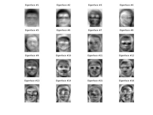
To plot the first 16 eigenfaces:

figure; hold on;
for i=1:min(16, size(eigenface.W,2))
    subplot(4,4,i);
    comp = cvtGray(eigenface.W(:,i), width, height);
    imshow(comp);
    title(sprintf("Eigenface #%i", i));
endfor

Resulting in:

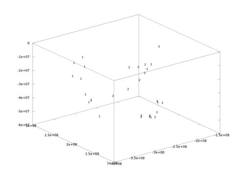
By plotting the whole stuff in 3D (just three classes here):

figure; hold on;
for i = findclasses(eigenface.y, [1,2,3])
    plot3(eigenface.P(1,i), eigenface.P(2,i), eigenface.P(3,i), 'r.');
    text(eigenface.P(1,i), eigenface.P(2,i), eigenface.P(3,i), num2str(eigenface.y(i)));
end

you can see that the faces are well seperated:

Accuracy

If you want to know the performance of the model I suggest using my framework at https://github.com/bytefish/facerec. There are functions for performing cross validations, see validation_example.m for their usage. The accuracy on the AT&T database is 96.25% with 30 eigenvectors.

If you want to calculate it yourself, here is how I did it with facerec:

% load function files from subfolders aswell
addpath (genpath ('.'));

% load data
[X y width height names] = read_images('/path/to/att');

% Learn Eigenfaces with 100 components
fun_eigenface = @(X,y) eigenfaces(X,y,30);
fun_predict = @(model, Xtest) eigenfaces_predict(model,Xtest,1);

% a Leave-One-Out Cross Validation (debug)
cv0 = LeaveOneOutCV(X,y,fun_eigenface, fun_predict, 1)

Feel free to play around with the code.